Charpy Impact Test Data

By Bill Amend

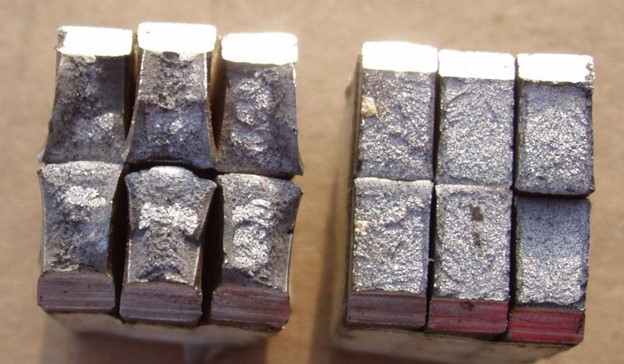
Two sets of Charpy specimen fracture surfaces showing how fracture appearance changes with test temperature

What is a Charpy Test?

A Charpy impact test evaluates the response of a notched steel specimen to impact loading.  The standard specimen size is 55 mm long x 10 mm x 10 mm, with a 2 mm deep vee notch machined into one side.  If the pipe wall is less than 10 mm thick, then a subsize specimen can be used in which the side with the notch is less than 10 mm high but preferably as close to full pipe wall thickness as possible. The specimen is supported at the ends, and the side opposite the notch is impacted by a swinging pendulum. The energy required to break the specimen is directly related to how high the pendulum continues to swing after impact with the specimen. The difference between the initial and the final pendulum height is translated to the absorbed energy.  Absorbed energy is measured in Joules or ft-lbs.  The greater the absorbed energy, the tougher the steel is.

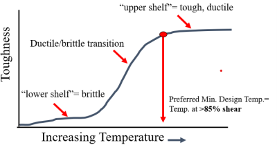
The second measurement that is made is based on a visual examination of the fracture surface.  The fracture surface shows indications indicative of either brittle (cleavage) or ductile (shear) failure or a mix of both.  Both fracture appearance and the absorbed energy are temperature related, and both relate to the performance of pipe in service.  When graphed, the shape of the temperature versus absorbed energy curve or the temperature versus %shear curve is not linear.  Instead, both typically follow a somewhat distorted “S” shape with very little change in apparent toughness at the extremes of high or low test temperatures, i.e., the so-called “upper shelf” and “lower shelf” energies, but relatively rapid changes in apparent toughness versus temperature at intermediate temperatures.

How Does the Charpy Test Compare to Pipe Performance?

The ability of a stressed pipe or pressure vessel to tolerate planar, crack-like flaws is much lower at temperatures that produce brittle failure. For brittle pipe, the likelihood of a long rupture is also greater than for a tough pipe having the same flaw size. Therefore, it is common to require that pipe and piping fittings operate at temperatures above the DBTT.  Superficially, the measurement of the DBTT would seem to be easy, but there are some complicating factors. First, keep in mind that the Charpy test evaluates response to dynamic loading, whereas quite often, pipeline flaws fail as a result of quasi-static (i.e., very slow) loading.  To compensate for the differences in response to dynamic vs. quasi-static loading, the test temperatures can be adjusted to make the Charpy specimen simulate what would be expected from quasi-static loading.  Secondly, a Charpy specimen, taken from a thick pipe, will overestimate the %shear that will occur on a thick pipe wall.   Recall that the Charpy specimen is never thicker than 10 mm (~0.394 in.).  The Charpy specimen can therefore overestimate the amount of shear expected on a thick pipe if the pipe wall is a lot thicker than 10 mm.  Additional temperature corrections can be applied so that the “small” Charpy specimen more closely replicates the %shear that can be expected on a “thick” pipe wall fracture.

Strategies for Selecting Test Temperatures

Pipe and fitting specifications often specify specific test temperatures to be used. Often, those temperatures are equal to either the design temperature, or 0°C.  Additional test temperatures can be used to better determine the relationship of operating temperature (or design temperature) to the temperature at which the steel transitions from tough, ductile behavior to brittle behavior, i.e. the ductile-to-brittle transition temperature (DBTT), or to determine the upper shelf energy or the lower shelf energy, or both.  In the pipeline industry the DBTT is commonly defined to be the temperature at which 85% shear is present on the fracture surface. Calculations can be performed to estimate how a Charpy specimen will perform at a new temperature based on data measured at a different temperature, or data can be graphed and interpolated, but as the difference in the two temperatures increases, the uncertainty in the calculated result also increased.  Therefore, it can be instructive to test specimens at the worst-case expected operating temperature, plus at one or more temperatures near the estimated DBTT to confirm the estimates, plus at temperatures that correct for the difference between impact loading and response to dynamic loading.

For more information on test temperature corrections and Charpy data interpretation, join us at either of the upcoming webinars, “Introduction to Pipeline Steels” or “What the Lab or Manufacturer Test Results Mean for Your Pipeline”.

For more information regarding this blog topic, please join us in either of the following two webinars: “Pipeline Flaws and Degradation” or “What Do the Test Results from the Manufacturer Test Reports (MTRs) or Your Lab Mean for Your Pipeline?”

Or contact the author, Bill Amend, P.E. at [email protected]